This One Keyboard Shortcut in Google Sheets Will Change How You Edit Formulas

Creating Relative References in Google Sheets

Cell references in formulas in Google Sheets are relative by default, meaning they adapt according to their position in the spreadsheet. As a result, there's no need to use F4 just yet, but we'll come to this soon.

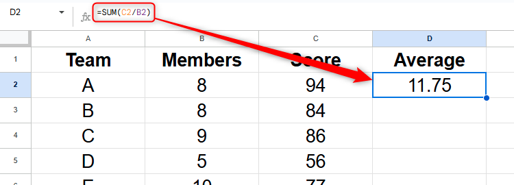
In this example, typing:

=SUM(C2/B2)

into cell D2 and pressing Enter divides team A's score by the number of members to produce an average member score.

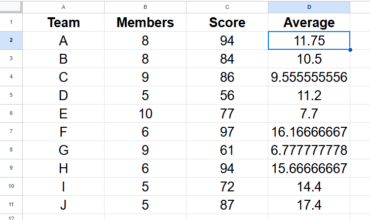
Because the references to cells C2 and B2 in this formula are relative—in other words, the formula references the cells that are one and two places to the left of the active cell, respectively—when you apply the formula to the remaining cells in the column by clicking and dragging the fill handle in the bottom-right corner of cell D2 downwards, the references adjust to perform the same calculation in each respective row.

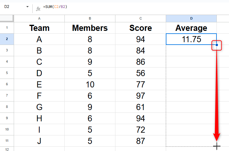
Google Sheets may even offer to complete this automatic filling process for you.

Alternatively, to speed up this process even further, rather than clicking and dragging the fill handle, double-click it. This forces Google Sheets to repeat the formula in every cell that contains data in an adjacent cell.

Copying the formula from the formula bar at the top of the Google Sheets window and pasting it into another cell duplicates the formula exactly as it is. In other words, the references won't change relative to the destination cell's position, so you need to work within the spreadsheet itself to ensure relative referencing works as expected.

In fact, no matter where the content of the copied cell is duplicated in this or another worksheet, it will always divide the value in the cell that's one to the left of the active cell by the value in the cell that's two to the left of the active cell.

Finally, to tidy up the number formatting, select all the resultant cells and click the "Decrease Decimal Places" button on the ribbon until you're happy with how your data is presented.

Using F4 to Create Absolute References in Google Sheets

As their name suggests, absolute references in Google Sheets remain fixed, even when they're moved or copied to different locations in the spreadsheet.

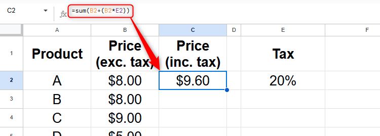
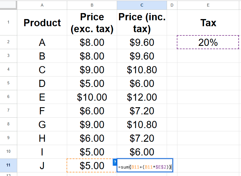
Imagine you've been tasked with working out the overall cost of ten products after tax is added.

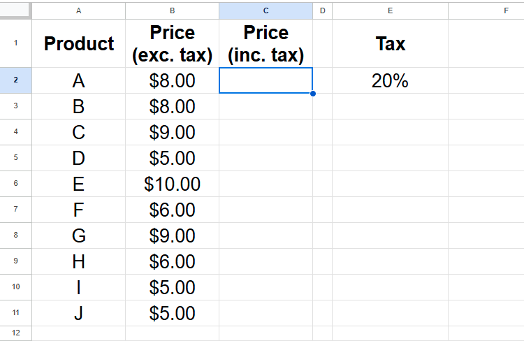
To do this, in cell C2, type:

=SUM(B2+(B2*E2))

and press Enter.

However, when you apply this formula to the remaining cells in column C by double-clicking the fill handle in cell C2, it doesn't work as expected. This is because each time the formula moves down a row, so do all its cell references.

For example, in cell C3, rather than referencing the tax rate in cell E2, the formula references cell E3, which is blank.

=SUM(B3+(B3*E3))

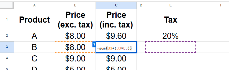
Instead, you only want the reference to the cell in column B to adjust according to the row it's on, with the reference to E2 remaining fixed.

To do this, first, head back to the original cell containing the formula (in this case, cell C2), and press F2 to enter cell edit mode. Then, use your arrows to move the cursor directly next to or within the E2 reference, and press F4. Notice how dollar signs are added to both the column and row reference to cell E2.

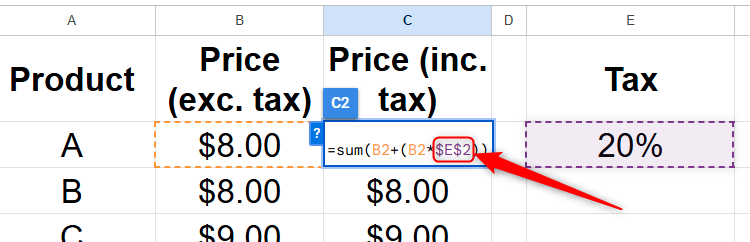
This means that what was previously a relative reference has now been converted into an absolute reference, so it will always remain the same no matter where the formula is duplicated in the spreadsheet.

Next time, rather than re-entering the cell, press F4 immediately after you've typed a reference in a formula to turn it into an absolute reference as you go.

Now, press Enter to confirm the edited formula, and click and drag the fill handle in cell C2 downwards to replace the incorrect formulas in the remaining cells in column C with the correct ones.

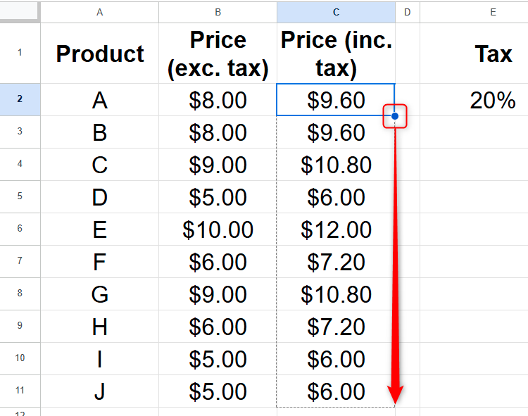
Double-click any of the resultant cells to check that the formula works as expected with the absolute reference to cell E2.

Using F4 to Create Mixed References in Google Sheets

The final reference type in Google Sheets is mixed references, which contain both a relative reference and an absolute reference at the same time. These are useful when you want to fix a column reference but leave the row reference adaptable, or vice versa. Let's look at an example of each.

Mixed References: Fixing the Column Reference Only

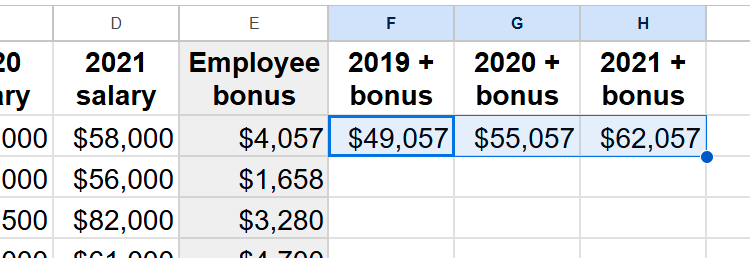
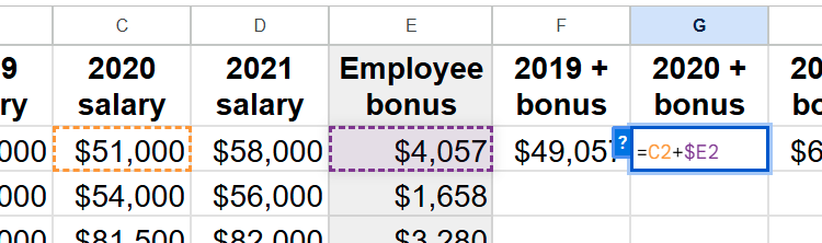
In this example, let's say you need to work out each employee's total salary over three years with bonus payments included.

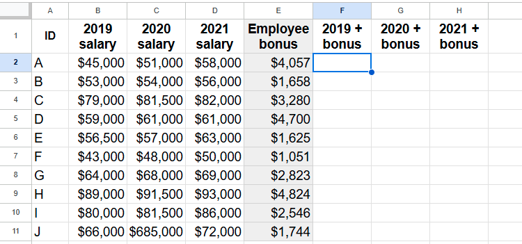
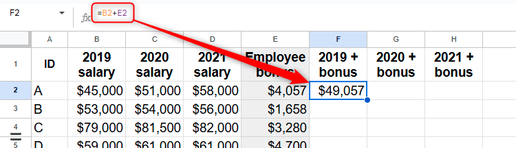
Start by typing the first formula in cell F2 to work out the total payment to employee F in 2019, and pressing Enter. In this case, it's:

=B2+E2

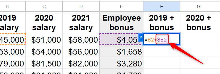
Now, before you go ahead and start duplicating this formula, let's review each part to work out which parts need to be relative and which parts need to be absolute:

• B: The reference to column B needs to be relative, so that when you duplicate the formula from column F to columns G and H, the formula correctly calculates the total payment for 2020 and 2021, respectively.
• 2: The reference to row 2 must also be relative, as you want the references in the formulas to adapt for each employee's details as you move down the rows.
• E: Every reference to cells in column E must not change, even when you duplicate the formula from column F to columns G and H, so this must be an absolute reference.
• 2: As with the previous reference to row 2, this needs to be relative so that it applies to each employee's figures.

So, in summary, you need the reference to column E in each formula to be absolute, with all other references remaining relative.

To do this, double-click cell F2 to enter cell edit mode. Then, place the cursor within or next to the reference to cell E2, and press F4 (three times) until only the reference to column E is preceded by the $ symbol.

=B2+$E2

Next, press Enter to commit the formula, and click and drag the fill handle from cell F2 to cell H2 to complete the calculations for employee A.

To check that the mixed reference has worked as expected, double-click cell G2 and verify that the correct precedent cells are highlighted—in this case, cells C2 and E2.

Now, finalize your data by selecting cells F2 to H2 and double-clicking the fill handle to duplicate this formula down the remaining rows.

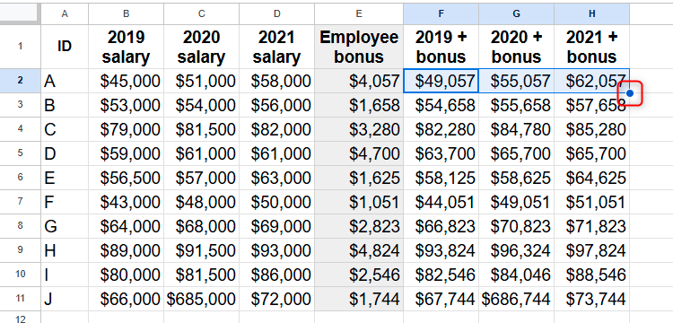
Once again, double-click any cell to confirm that the formula it contains references the correct cells.

Mixed References: Fixing the Row Reference Only

In a final example, your aim is to determine how much money each shop is projected to make based on the expected annual growth rate.

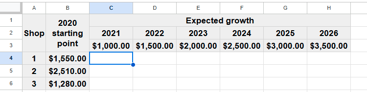
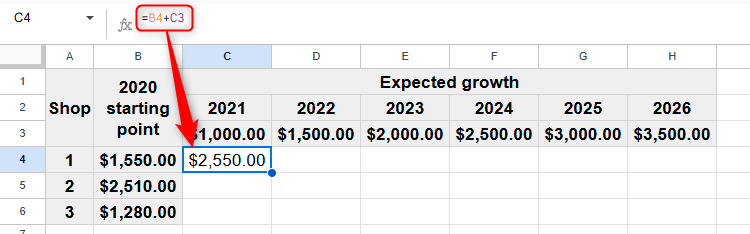
As always, start by typing the first formula, and work out from that point what needs to be relative and what needs to be fixed. In this case, in cell C4, type:

=B4+C3

to add the 2020 starting point for shop 1 to the expected growth for 2021.

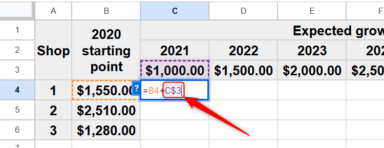
Now, let's review the references in this formula:

• B: This column reference needs to be relative, as you want the total to be cumulative as you move across the row, adding each yearly total to the following year's expected growth.
• 4: This row reference also needs to be relative, as you want the reference to change according to the row it's on.
• C: As with the reference to column B, the reference to column C needs to be relative, to allow for cumulative growth.
• 3: The reference to row 3 needs to be absolute, however, because this row contains the expected growth for each shop each year.

So, place your cursor in or next to the reference to cell C3, and press F4 (twice) until the dollar sign appears before the reference to row 3.

=B4+C$3

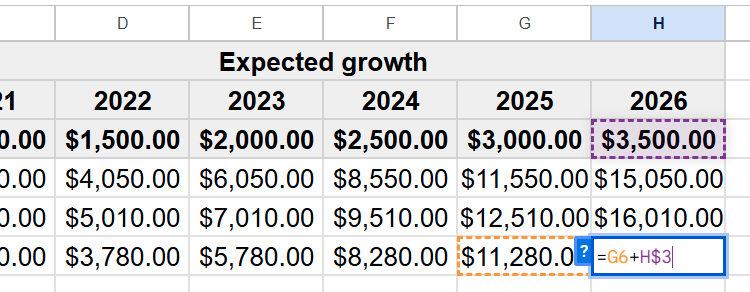
Finally, apply the formula to the remaining cells in the range using the fill handle, and double-click a random cell to check that the mixed reference works as expected.

---

If you're deciding whether you should use Google Sheets or Microsoft Excel, there are several key differences between the two programs that you should consider. For example, Excel is known for offering more advanced data analysis tools, but real-time collaboration in Sheets works more seamlessly. However, regardless of which one you choose, knowing how relative, absolute, and fixed references work is key to generating formulas that work as expected.