How to Use the IMPORTRANGE Function to Import Data From One Google Sheets File Into Another

The IMPORTRANGE function in Google Sheets has two arguments:

=IMPORTRANGE(a,b)

Argument a is the link (URL) to the Google Sheets file where the range you want to import is located—enclosed in double quotes—or a reference to a cell containing the URL.

Argument b is the reference to the range. This can be cell references, a sheet name followed by cell references, a named range, a table name, or a column within a table—all of which must be in double quotes. Argument b can also reference a cell containing the cell references of the source data, and this doesn't need quotation marks.

Confused? Let's explore each of these more closely.

Importing Data Using Direct Cell References

You can import data from one Google Sheets file to another by specifying the source URL and the relevant cell references. This is useful if you're sure that the source data won't change location or grow in size.

Let's imagine you have two Google Sheets files open on separate browser tabs—File 1 contains a list of names in cells A2 to A11 that you want to import into File 2.

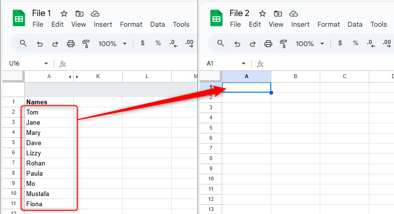
To do this, select the cell in File 2 where you want the list to be imported into, type the following formula—remembering to enclose both the URL and cell references in quotation marks—and press Enter:

=IMPORTRANGE("https://docs.google.com/spreadsheets/d...","A2:A11")

The example formulas in this guide only show part of the URL for demonstration purposes. In your case, make sure you insert the whole URL into the formula.

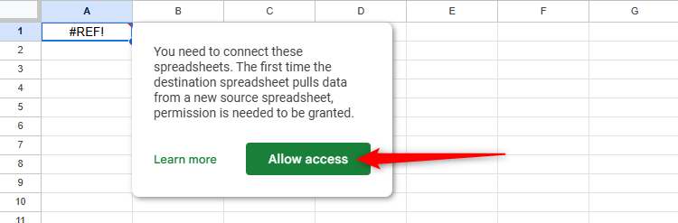
The first time you connect the active and referenced worksheets, you may see a #REF! error. If you do, hover over the cell containing the error to see one of two messages.

On the one hand, if you own both spreadsheets, Google Sheets will tell you that you need to grant permission to link the files. To do this, click "Allow Access."

On the other hand, if you don't own the source spreadsheet and haven't been given edit access, you'll be told that you don't have permission to use the linked sheet in your IMPORTRANGE formula. In this case, paste the URL into your browser's URL bar, click "Request Edit Access," and wait for the owner to grant this request.

Once the correct permissions are activated, the range is imported successfully.

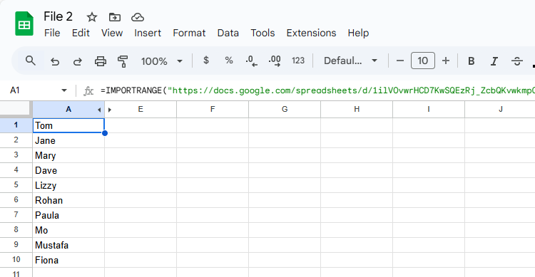
What's more, any changes to the content of cells A2 to A11 in File 1 will be reflected in the imported data in File 2 after it refreshes automatically.

If the source data expands or changes location, the cell reference you used in argument b won't adjust to this change, so you'll need to adjust the formula accordingly.

By default, the IMPORTRANGE function imports from the first worksheet in the specified file, even if you use the URL of a different worksheet in the file. However, if you want to import a range from another worksheet, for argument b, type the sheet name, followed by an exclamation mark, and then the cell references.

For example, this formula would import the data from cells A2 to A11 in Sheet 2 of the source file:

=IMPORTRANGE("https://docs.google.com/spreadsheets/d...","Sheet2!A2:A11")

Pro Tip: Importing Data From Within the Same Google Sheets File

The IMPORTRANGE function is intended to import ranges from different Google Sheets files. To import data from one spreadsheet in a Google Sheets file to another spreadsheet in the same Google Sheets file, use the ARRAYFORMULA function. For example, typing:

=ARRAYFORMULA(A2:A11)

dynamically copies the data from cells A2 to A11 in the same worksheet.

Similarly, typing:

=ARRAYFORMULA(Sheet1!A2:A11)

into a cell in Sheet 2 duplicates the data in cells A2 to A11 in Sheet 1.

Importing Data Using Indirect References

In the examples above, argument a contains the full URL of the source data, leading to lengthy formulas that are challenging to parse. Instead, to make the formula tidier, you could reference a cell that contains the source URL.

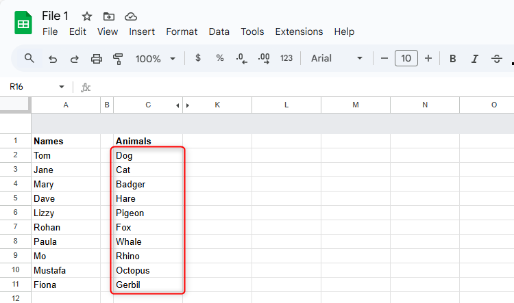
Here, cells C2 to C11 in File 1 contain a list of animals you want to import into File 2.

If you have edit access to File 1, copy its URL, and select a blank cell in File 2. Then, click the formula bar at the top of the spreadsheet so that the cursor is flashing, and press Ctrl+V (or right-click and select "Paste"), before pressing Enter.

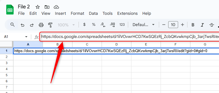
If you paste the link directly into the cell, Google Sheets reformats the link, causing it to be incompatible with the IMPORTRANGE function. This is why it's best practice to paste the URL into the formula bar after selecting the destination cell.

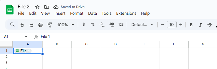
Next, select the cell where you just pasted the link, and click "Chip."

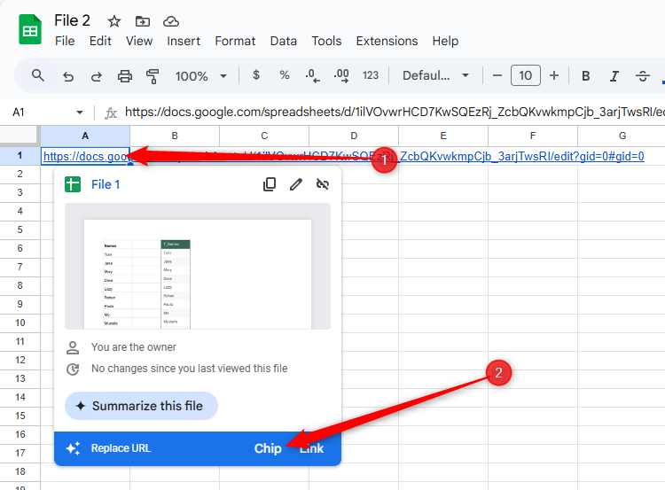
This shortens the link into a file label, making your spreadsheet tidier and more professional.

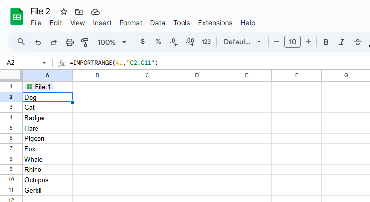
Then, in another cell in File 2, type:

=IMPORTRANGE(A1,"C2:C11")

where A1 is the cell in File 2 containing the URL of File 1 that you just pasted, and C2:C11 is the range in File 1 that you want to import.

The cell containing the URL doesn't need to be in quotation marks.

Then, press Enter.

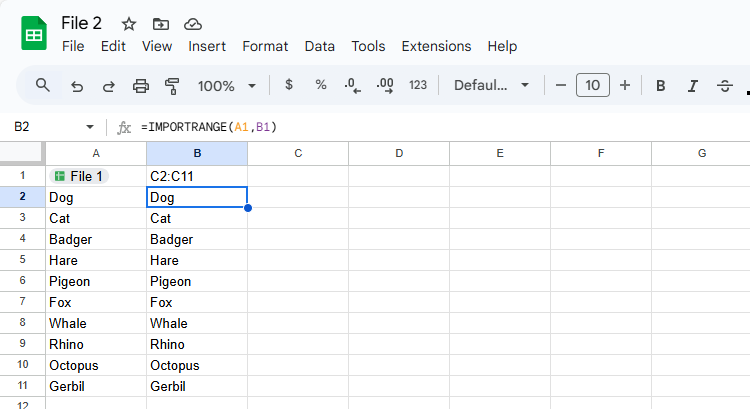
Rather than hard-coding the cell references in argument b, you can type these into a separate cell in File 2, and reference that instead. As well as further shortening your formula, this method means that you can easily change the reference without having to edit the formula itself.

In this example, the formula:

=IMPORTRANGE(A1,B1)

in cell B2 takes the URL from cell A1, and the cell references from cell B1.

If you later realize that you want the imported range to be static (rather than allowing it to update according to the source data), simply select and copy the range, and press Ctrl+Shift+V to paste the data as values.

Importing Data From Named Tables and Ranges

The IMPORTRANGE function in Google Sheets can also import tables, columns in tables, and ranges.

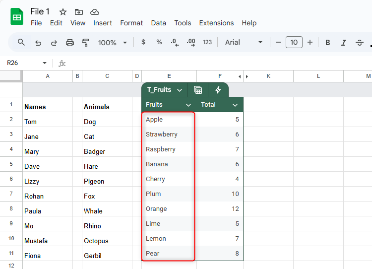
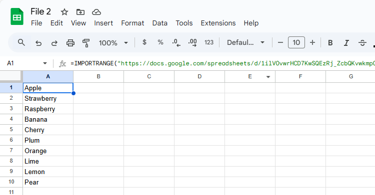
In this example, File 1 contains a table named T_Fruits, and you want to import the column named Fruits into File 2.

So, after ensuring you have edit access to File 1, in a blank cell in File 2, type:

=IMPORTRANGE("https://docs.google.com/spreadsheets/d...","T_Fruits[Fruits]")

where the URL is the link to File 1, T_Fruits is the name of the table, and Fruits is the column within that table that you want to import.

If you type only the name of the table (and not a column header), the whole table will be imported.

The benefit of this approach is that if more rows are added to the data, the IMPORTRANGE function will pick these up, meaning the changes will be reflected in the imported version. That said, if you rename the table or column headers, you'll need to update argument b of the IMPORTRANGE formula accordingly.

In a similar fashion, argument b can also be a named range.

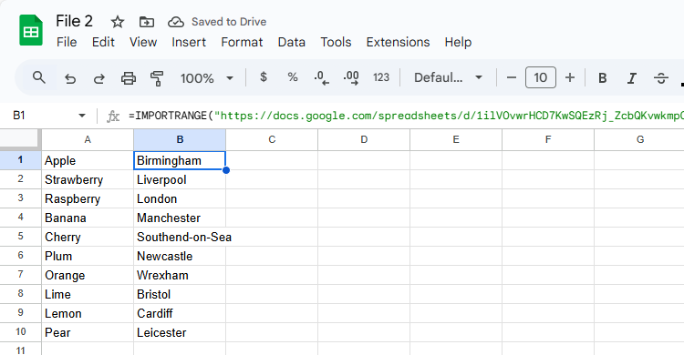
For example, cells H2 to H11 in File 1 are named R_Cities.

As a result, the formula in File 2 can import this data by referencing the named range:

=IMPORTRANGE("https://docs.google.com/spreadsheets/d...","R_Cities")

Nesting IMPORTRANGE in Other Functions

IMPORTRANGE doesn't have to be used on its own in Google Sheets—it can also be used alongside other formulas to perform calculations on data in other Google Sheets files.

In this example, let's imagine File 1 has a list of scores in cells J2 to J6. Your aim is to use the IMPORTRANGE function with the SUM function to evaluate these cells, sum their values, and return the result in File 2.

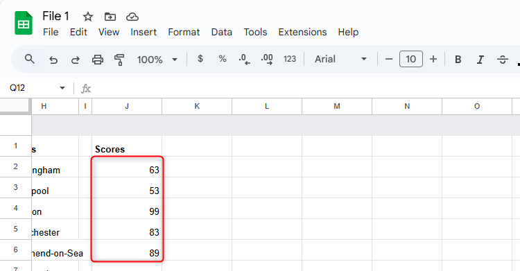
To do this, in a blank cell in File 2, type:

=SUM(IMPORTRANGE("https://docs.google.com/spreadsheets/d...","J2:J6"))

where the IMPORTRANGE function references cells J2 to J6 in File 1, and the SUM function adds the values they contain.

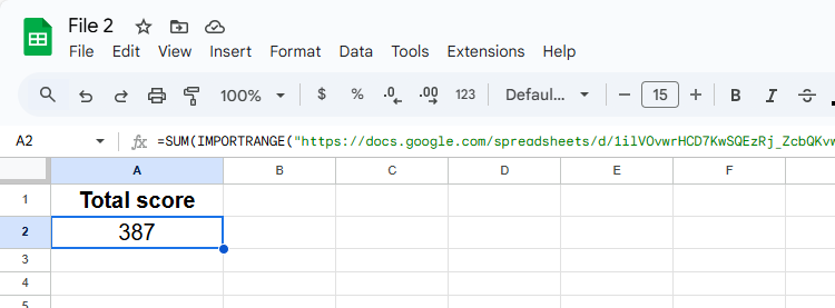
According to Google, using this approach is faster than first using IMPORTRANGE to import the data, and then using a separate SUM function to sum the imported range.

The IMPORTRANGE function can't reference a cell that contains another volatile function—like NOW or the random number functions RAND and RANDBETWEEN—as doing so would potentially overload the spreadsheet's resources. The only exception is the TODAY function, since this only updates once daily.

Points to Note When Using the IMPORTRANGE Function

Before you go ahead and use IMPORTRANGE in your Google Sheets spreadsheets, here are some final pointers to bear in mind:

• References and names in IMPORTRANGE don't update: If the range reference, table name, column name, or range name changes, it needs to be updated in the IMPORTRANGE formula in the destination file.
• You can create an IMPORTRANGE chain: For example, you could use the function in File 2 to reference a range in File 1, and then use it again in File 3 to reference the imported range in File 2. That said, you should try to limit these chains, as having too many could affect the performance of your spreadsheets.
• IMPORTRANGE requires an internet connection: Since this is an external data function, it needs an internet connection to work. A slower internet connection will result in importing lags.
• Imports are capped at 10MB: The IMPORTRANGE function is limited to importing up to 10MB per data request. This limit is in place to reduce the adverse effect the function has on performance and resources.

---

Because it's an online software, many prefer Google Sheets to its desktop competitors, such as Microsoft Excel. Indeed, to perform the same importing actions in Excel, you would need to use the Power Query Editor tool, a route that requires many more steps.